


Introduction to Graph Theory in C++
_author: TatoNaranjo
Table of Contents
What is a graph?
Graphs are typically used to represent images or wireless signals, but a more popular representation could be a map. Imagine a map that has several cities connected to each other by roads.
Some of the questions we could ask ourselves would be:
- Is city A connected to city B?
- What is the shortest distance to travel from city A to city B?
A graph can be seen as a relationship between objects. Let’s look at the following example: Imagine you have a network of friends where you know who knows who and who doesn’t.
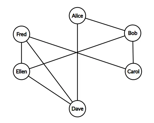
We can see that if Bob is friends with Alice, Alice is also friends with Bob, so there is a friendship relationship
Graph Terminology
A graph consists of nodes and edges. Nodes are numbered using integers [1,2,...,n].
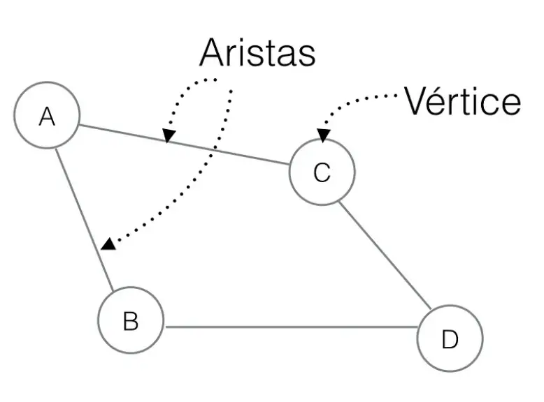
This graph is composed of 4 nodes and 4 edges.
A path leads a node a to a node b through the edges. For example, the following graph has a path 1->3->4->5 of length 3 from node 1 to node 5.
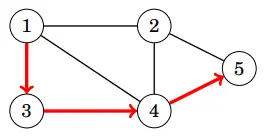
1 -> 3 -> 4 -> 5
In turn, a path becomes a cycle if the first and last nodes are the same. It is also considered a simple path if each node appears at least once in the route.
Connectivity
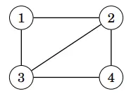
A graph is connected if there is a path between any two nodes. For example, the following graph is connected.
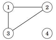
The following graph is not connected, since it is not possible to connect node 4 with any other node.
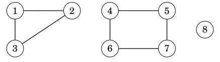
The connected parts of a graph are called components. For example, the following graph contains three components {1,2,3}, {4,5,6,7} and {8}.
A Tree is a connected graph if it consists of n nodes and n-1 edges. There is a unique path between any two nodes of a tree. For example, the following graph is a tree.
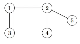
Edge Directions
A graph is directed if the edges can be traversed in only one direction. For example, the following graph is directed:
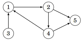
The graph above contains a path 3->1->2->5 from node 3 to node 5, but there is no path from node 5 to node 3.
Edge Weights
In a weighted graph, each edge is assigned a weight. Weights are commonly interpreted as edge lengths. For example, the following is a weighted graph.
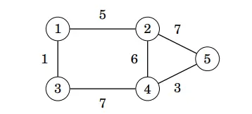
The length of a path in a weighted graph is made up of the sum of the edge weights for each path. In the previous example, we can see that the length of the path 1->3->4->5 is 11. This last path is the shortest path from node 1 to node 5.
Neighbors and Degrees
Two nodes are neighbors or adjacent if there is an edge connecting them to each other. The degree of a node is the number of neighbors it has.
For example, in the following graph the neighbors of node 2 are 1,4 and 5. So it’s a degree 3 node.
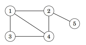
The sum of degrees in a graph is always 2m, where m is the number of edges, because each edge increases the degrees of exactly two nodes by one. For this reason, the sum of degrees is always even.
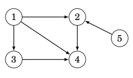
In a directed graph, the in-degree of a node is the number of edges ending at that node, while the out-degree is the number of edges starting at that node.
How to Represent Graphs in an Algorithm
There are many ways to represent graphs in an algorithm. The choice of a data structure depends on the size of the graph and how the algorithm processes the data.
Below I will leave you the three most common representations, using the C++ language.
Adjacency List
In the adjacency list representation, each node x in the graph is assigned an adjacency list consisting of the nodes that have an edge connecting to node x.
Adjacency lists are the most popular way to represent graphs, and most algorithms can be implemented efficiently using them.
A convenient way to store adjacency lists is by declaring an array of vectors:
vector<int> adj[N];The constant N is chosen such that all adjacency lists can be stored. For example, the graph:
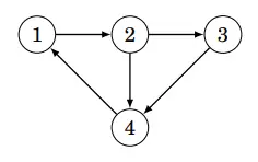
Can be saved as follows:
adj[1].push_back(2);
adj[2].push_back(3);
adj[2].push_back(4);
adj[3].push_back(4);
adj[4].push_back(1);
For a weighted graph the structure extends as follows:
vector<pair<int,int>> adj[N];In this case the adjacency list of a node a always contains the pair {b,w}, where there is an edge from node a to a node b with weight w.
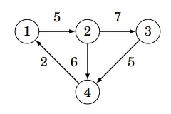
Can be saved as follows:
adj[1].push_back({2,5});
adj[2].push_back({3,7});
adj[2].push_back({4,6});
adj[3].push_back({4,5});
adj[4].push_back({1,2});
The benefit of using adjacency lists is that we can efficiently find the nodes we can move to via a given node via an edge:
for(auto g: adj[s]){
  // Process node g
}
Adjacency Matrix
An adjacency matrix is a two-dimensional array that indicates which edges a graph has. We can efficiently check from an adjacency matrix if there is a vertex between two nodes. The matrix can be saved as an array:
int adj[N][N];Where each value adj[a][b] indicates if the graph contains an edge from node a to node b. If the edge is included in the graph, then adj[a][b] = 1, otherwise adj[a][b] = 0.
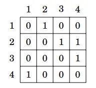
If the graph is weighted, the adjacency matrix representation can be extended so that the matrix contains the edge weight:
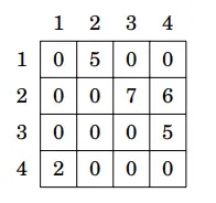
The problem with the adjacency matrix is that the matrix contains n^2 elements, and usually many of these are zero. For efficiency and algorithm performance reasons, the representation cannot be used if the graph is very large.
Edge List
An edge list contains all the edges of a graph in an order. This is a convenient way to represent a graph if the algorithm processes all the edges of a graph and there is no need to find edges starting at a given node.
The edge list can be stored in a vector:
vector<pair<int,int>> aristas;For example:
aristas.push_back({1,2});
aristas.push_back({2,3});
aristas.push_back({2,4});
aristas.push_back({3,4});
aristas.push_back({4,1});
If the graph is weighted, the structure extends to:
vector<tuple<int,int,int>> aristas;Each element in this list is of the form (a,b,w), indicating that there is an edge from node a to node b and has a weight of w.
aristas.push_back({1,2,5});
aristas.push_back({2,3,7});
aristas.push_back({2,4,6});
aristas.push_back({3,4,5});
aristas.push_back({4,1,2});